Ok, this is a continuation of two streams of articles here, first my recent NETCONF tutorial here, and secondly my very old project (back then in Java) of visualization of network topologies using SNMP information called “HelloRoute”. So this is a resurrection of a very old ideas, just using newer methods and tools. But first a foreword on visualization.
Foreword – Visualization use in Network Infrastructure by Author’s experience
Well, as far as I would say, automated network visualization or documentation never really took of as primary source of documentation, everywhere I look we still maintain manually created maps with version control, trying to keep them up-to-date in change process and etc… , the reason why this is so is the context that human author can give the map, for example office networks mapped by purpose or parts of buildings, or by legal organizations. Have a look on the picture below, this is a difference between human and automated maps in most generic network modeling tools.
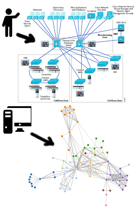
Human vs computer generated network diagrams
Now to not completely kill the point of you finishing this tutorial, I BELIEVE THE PROBLEM IS THAT VISUALIZATION TOOLS ON MARKET ARE MOSTLY GENERIC PRODUCTS, by this I mean they have generic algorithms, only follow what the vendor could “expect” in advance and there are not many ways how to add extra code/logic to them to fit YOUR visualization context without paying $$$ to the vendor. So from my perspective the for any network infrastructure maintenance organization (e.g. myself working in my job or freelance consultancy) the SOLUTION IS TO BUILD VISUALIZATION TOOLS IN-HOUSE using available components (libraries, algorithms) on the fly and not put forward generic vendor software if they cannot be heavily customized (and I am yet to find such vendor).
What we will build in this tutorial then?
Simple, we will build something like this, which is a middle-ground between the two extremes, or at least for my small Spine-Leaf network( LIVE DEMO link HERE ):
This is not the best visualization in the world (I do not claim that), the point here is to try to show you that building something yourself is not that hard as it seems with a little bit of scripting.
Part I. LAB topology and prerequisites
We will continue exactly where we left last time in the NETCONF tutorial and re-iterate the same LAB and requirements.
A. LAB Topology
Simple as last time, I am having my development laptop with SSH/IP access to two comware7 switches, those in turn have some LLDP neighbors on both uplinks and server downlinks.
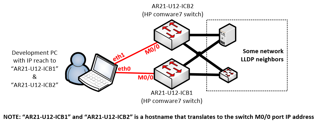
LAB Topology is simply active two comware7 switches with IP management access
NOTE: Yes, servers speak LLDP and from my perspective is a good practice to have that running, on both Windows and Linux this is a few clicks/commands work to enable and also hyper-visors in DCs can have it, for example on ESX/vmWare’s distributed switch settings, this is one checkbox to have enabled.
B. Installed python + libraries
I will be using python 2.7 interpreter, so download that for your system (preferred linux so that installation is simple) and download/install both ncclient library using pip and the HP Networkings PyHPEcw7 library using a few commands below:
# Install ncclient
pip install ncclient

# Install HPN's pyhpecw7 library
git clone https://github.com/HPENetworking/pyhpecw7.git
cd pyhpecw7
sudo python setup.py install
C. (Optional) Web development tools plugin
When we get to developing the visualization, we will be using simple HTML/CSS + Javascript, you only need a notepad to work on this, but for troubleshooting, I really recommend that you googlesearch “Web development tools” plugin for your browser or at least learn where your particular browser have “console” view so you can see what the Javascript prints to the console as debug messages during problems.
Part II. Example python script to pull LLDP neighbors to a JSON map
Using the knowledge you gained in my previous NETCONF tutorial, you should be able to understand what is happening here, so I will just put the whole code here, and provide some explanation afterwards. But I will not go through this line-by-line as this is NOT a python tutorial (other pages for that). The code essentials:
INPUT: Needs “DEVICES.txt” file to exist nearby that has list of IPs/Hostnames to access, one host at each line, e.g. I have inside my DEVICES.txt:
AR21-U12-ICB1
AR21-U12-ICB2
OUTPUT: Then the script will product three JSON files, these are:
- graph.json – Main topology file, that will hold in JSON format all the graph nodes (devices) and links (interfaces), we will alter use this as input to visualization
- no_neighbor_interfaces.json – This is a bonus JSON file that I decided to create to have available also a quick list of interfaces that are in “UP” operational status, but there is no LLDP neighbor behind them, this is an “unknown factor” risk I want to be aware of in my visualization exercise
- neighborships.json – This describes per-device a list of interfaces and LLDP neighbor behind each of them.
SCRIPT SOURCE:
#!/bin/python
from pyhpecw7.comware import HPCOM7
from pyhpecw7.features.vlan import Vlan
from pyhpecw7.features.interface import Interface
from pyhpecw7.features.neighbor import Neighbors
from pyhpecw7.utils.xml.lib import *
import yaml
import pprint
import json
import re

##########################
# CONFIGURATION OF ACCESS
##########################
USER="admin"
PASS="admin"
PORT=830

#########################################################
# REGULAR EXPLRESSIONS FOR MATCHING PORT NAMES TO SPEEDS
# NOTE: This is used in visuzation later to color lines
#########################################################
LINK_SPEEDS = [ ("^TwentyGigE*","20"),
                ("^FortyGig*","40") ,
                ("^Ten-GigabitEthernet*","10") ,
                ("^GigabitEthernet*","1")  ]

#########################################################
# REGULAR EXPLRESSIONS FOR MATCHING DEVICES HIERARHY
# E.g. Access layer switches have "AC" in their name
# or aggregation layer devices have "AG" in their names
#########################################################
NODE_HIERARCHY = [ ('.+ICB.*',"2"),
                   ('^[a-zA-Z]{5}AG.*',"3"),
                   ('^[a-zA-Z]{5}AC.*',"2"),
                   ('^[a-zA-Z]{5}L2.*',"4") ]

####################
# Connection method
####################
def connect(host,username,password,port):
  args = dict(host=host, username=username, password=password, port=port)
  print("Connecting " + host)
  # CREATE CONNECTION
  device = HPCOM7(**args)
  device.open()
  return device

################################
# Returns RAW python Dictionary
# with Neighbor NETCONF details
#################################
def getNeighbors(device):
  print 'getNeighbors'
  neighbors = Neighbors(device)
  neigh_type=dict(default='lldp', choices=['cdp', 'lldp'])
  response = getattr(neighbors, "lldp")
  results = dict(neighbors=response)
  clean_results = list()

  for neighbor in results['neighbors']:
    if str(neighbor['neighbor']) == "None" or str(neighbor['neighbor']) == "":
      print("Removing probably bad neighbor \""+ str(neighbor['neighbor']) + "\"");
    else:
      clean_results.append(neighbor)

  return clean_results

###############################################
# Takes RAW Dictionary of Neighbors and returns
# simplified Dictionary of only Neighbor nodes
# for visuzation as a node (point)
#
# NOTE: Additionally this using RegEx puts layer
# hierarchy into the result dictionary
###############################################
def getNodesFromNeighborships(neighborships):
  print "getNodesFromNeighborships:"
  nodes = {'nodes':[]}
  for key,value in neighborships.iteritems():
    print("Key:" + str(key) + ":")

    '''
    PATTERNS COMPILATIOn
    '''
    print ("Hostname matched[key]: " + key)
    group = "1" # for key (source hostname)
    for node_pattern in NODE_HIERARCHY:
      print ("Pattern: " + node_pattern[0]);
      pattern = re.compile(node_pattern[0]);
      if pattern.match(key):
        print("match")
        group = node_pattern[1]
        break
    print("Final GROUP for key: " + key + " is " +group)

    candidate = {"id":key,"group":group}
    if candidate not in nodes['nodes']:
      print("adding")
      nodes['nodes'].append(candidate)

    for neighbor in value:
      print("neighbor: " + str(neighbor['neighbor']) + ":")
      '''
      PATTERNS COMPILATIOn
      '''
      print ("Hostname matched: " + neighbor['neighbor'])
      group = "1"
      for node_pattern in NODE_HIERARCHY:
        print ("Pattern: " + node_pattern[0]);
        pattern = re.compile(node_pattern[0]);
        if pattern.match(neighbor['neighbor']):
          print("match")
          group = node_pattern[1]
          break
      print("Final GROUP for neighbor: " + key + " is " +group)


      candidate2 = {"id":neighbor['neighbor'],"group":group}
      if candidate2 not in nodes['nodes']:
        print("adding")
        nodes['nodes'].append(candidate2)

  return nodes

###############################################
# Takes RAW Dictionary of Neighbors and returns
# simplified Dictionary of only links between
# nodes for visuzation later (links)
#
# NOTE: Additionally this using RegEx puts speed
# into the result dictionary
###############################################
def getLinksFromNeighborships(neighborships):
  print "getLinksFromNeighborships:"

  links = {'links':[]}
  for key,value in neighborships.iteritems():
    print(str(key))
    for neighbor in value:

      '''
      PATTERNS COMPILATIOn
      '''
      print ("Interface matched: " + neighbor['local_intf'])
      speed = "1" # DEFAULT
      for speed_pattern in LINK_SPEEDS:
        print("Pattern: " + speed_pattern[0])
        pattern = re.compile(speed_pattern[0])

        if pattern.match(neighbor['local_intf']):
          speed = speed_pattern[1]

      print("Final SPEED:" + speed)

      links['links'].append({"source":key,"target":neighbor['neighbor'],"value":speed})

  return links

##############################################
# Filters out links from simplified Dictionary
# that are not physical
# (e.g Loopback or VLAN interfaces)
#
# NOTE: Uses the same RegEx definitions as
# speed assignment
##############################################
def filterNonPhysicalLinks(interfacesDict):

  onlyPhysicalInterfacesDict = dict()

  print "filterNonPhysicalLinks"
  for key,value in interfacesDict.iteritems():
    print("Key:" + str(key) + ":")
    onlyPhysicalInterfacesDict[key] = [];

    for interface in value:

      bIsPhysical = False;
      for name_pattern in LINK_SPEEDS:
        pattern = re.compile(name_pattern[0])

        if pattern.match(interface['local_intf']):
          bIsPhysical = True;
          onlyPhysicalInterfacesDict[key].append({"local_intf":interface['local_intf'],
                                                  "oper_status":interface['oper_status'],
                                                  "admin_status":interface['admin_status'],
                                                  "actual_bandwith":interface['actual_bandwith'],
                                                  "description":interface['description']})
          break;

      print(str(bIsPhysical) + " - local_intf:" + interface['local_intf'] + " is physical.")


  return onlyPhysicalInterfacesDict;

##############################################
# Filters out links from simplified Dictionary
# that are not in Operational mode "UP"
##############################################
def filterNonActiveLinks(interfacesDict):

  onlyUpInterfacesDict = dict()

  print "filterNonActiveLinks"
  for key,value in interfacesDict.iteritems():
    print("Key:" + str(key) + ":")
    onlyUpInterfacesDict[key] = [];

    for interface in value:
      if interface['oper_status'] == 'UP':
        onlyUpInterfacesDict[key].append({"local_intf":interface['local_intf'],
                                          "oper_status":interface['oper_status'],
                                          "admin_status":interface['admin_status'],
                                          "actual_bandwith":interface['actual_bandwith'],
                                          "description":interface['description']})
        print("local_intf:" + interface['local_intf'] + " is OPRATIONAL.")

  return onlyUpInterfacesDict;

################################################
# Takes RAW neighbors dictionary and simplified
# links dictionary and cross-references them to
# find links that are there, but have no neighbor
################################################
def filterLinksWithoutNeighbor(interfacesDict,neighborsDict):

  neighborlessIntlist = dict()

  print "filterLinksWithoutNeighbor"
  for devicename,neiInterfaceDict in neighborships.iteritems():
    print("Key(device name):" + str(devicename) + ":")

    neighborlessIntlist[devicename] = []

    for interface in interfacesDict[devicename]:
      bHasNoNeighbor = True
      for neighbor_interface in neiInterfaceDict:
        print("local_intf: " + interface['local_intf']
           + " neighbor_interface['local_intf']:" + neighbor_interface['local_intf'])
        if interface['local_intf'] == neighbor_interface['local_intf']:
          # Tries to remove this interface from list of interfaces
          #interfacesDict[devicename].remove(interface)
          bHasNoNeighbor = False
          print("BREAK")
          break;

      if bHasNoNeighbor:
        neighborlessIntlist[devicename].append(interface)
        print("Neighborless Interface on device: " + devicename + " int:" + interface['local_intf'])

  return neighborlessIntlist;

###########################
# Collects all Interfaces
# using NETCONF interface
# from a Device
#
# NOTE: INcludes OperStatus
# and ActualBandwidth and
# few other parameters
###########################

def getInterfaces(device):
  print 'getInterfaces'

  E = data_element_maker()
  top = E.top(
      E.Ifmgr(
          E.Interfaces(
            E.Interface(
            )
          )
      )
  )
  nc_get_reply = device.get(('subtree', top))

  intName = findall_in_data('Name', nc_get_reply.data_ele)
  ## 2 == DOWN ; 1 == UP
  intOperStatus = findall_in_data('OperStatus', nc_get_reply.data_ele)
  ## 2 == DOWN ; 1 == UP
  intAdminStatus = findall_in_data('AdminStatus', nc_get_reply.data_ele)
  IntActualBandwidth = findall_in_data('ActualBandwidth', nc_get_reply.data_ele)
  IntDescription = findall_in_data('Description', nc_get_reply.data_ele)

  deviceActiveInterfacesDict = []
  for index in range(len(intName)):

    # Oper STATUS
    OperStatus = 'UNKNOWN'
    if intOperStatus[index].text == '2':
      OperStatus = 'DOWN'
    elif intOperStatus[index].text == '1':
      OperStatus = 'UP'

    # Admin STATUS
    AdminStatus = 'UNKNOWN'
    if intAdminStatus[index].text == '2':
      AdminStatus = 'DOWN'
    elif intAdminStatus[index].text == '1':
      AdminStatus = 'UP'

    deviceActiveInterfacesDict.append({"local_intf":intName[index].text,
                                       "oper_status":OperStatus,
                                       "admin_status":AdminStatus,
                                       "actual_bandwith":IntActualBandwidth[index].text,
                                       "description":IntDescription[index].text})

  return deviceActiveInterfacesDict


###########################
# MAIN ENTRY POINT TO THE
# SCRIPT IS HERE
###########################
if __name__ == "__main__":
  print("Opening DEVICES.txt in local directory to read target device IP/hostnames")
  with open ("DEVICES.txt", "r") as myfile:
    data=myfile.readlines()

    '''
    TRY LOADING THE HOSTNAMES
    '''
    print("DEBUG: DEVICES LOADED:")
    for line in data:
      line = line.replace('\n','')
      print(line)


    #This will be the primary result neighborships dictionary
    neighborships = dict()

    #This will be the primary result interfaces dictionary
    interfaces = dict()


    '''
    LETS GO AND CONNECT TO EACH ONE DEVICE AND COLLECT DATA
    '''
    print("Starting LLDP info collection...")
    for line in data:
      #print(line + USER + PASS + str(PORT))
      devicehostname = line.replace('\n','')
      device = connect(devicehostname,USER,PASS,PORT)
      if device.connected: print("success")
      else:
        print("failed to connect to " + line + " .. skipping");
        continue;

      ###
      # Here we are connected, let collect Interfaces
      ###
      interfaces[devicehostname] = getInterfaces(device)

      ###
      # Here we are connected, let collect neighbors
      ###
      new_neighbors = getNeighbors(device)
      neighborships[devicehostname] = new_neighbors


    '''
    NOW LETS PRINT OUR ALL NEIGHBORSHIPS FOR DEBUG
    '''
    pprint.pprint(neighborships)
    with open('neighborships.json', 'w') as outfile:
      json.dump(neighborships, outfile, sort_keys=True, indent=4)
      print("JSON printed into neighborships.json")

    '''
    NOW LETS PRINT OUR ALL NEIGHBORSHIPS FOR DEBUG
    '''
    interfaces = filterNonActiveLinks(filterNonPhysicalLinks(interfaces))
    pprint.pprint(interfaces)
    with open('interfaces.json', 'w') as outfile:
      json.dump(interfaces, outfile, sort_keys=True, indent=4)
      print("JSON printed into interfaces.json")


    '''
    GET INTERFACES WITHOUT NEIGHRBOR
    '''
    print "====================================="
    print "no_neighbor_interfaces.json DICTIONARY "
    print "======================================"
    interfacesWithoutNeighbor = filterLinksWithoutNeighbor(interfaces,neighborships)
    with open('no_neighbor_interfaces.json', 'w') as outfile:
      json.dump(interfacesWithoutNeighbor, outfile, sort_keys=True, indent=4)
      print("JSON printed into no_neighbor_interfaces.json")

    '''
    NOW LETS FORMAT THE DICTIONARY TO NEEDED D3 LIbary JSON
    '''
    print "================"
    print "NODES DICTIONARY"
    print "================"
    nodes_dict = getNodesFromNeighborships(neighborships)
    pprint.pprint(nodes_dict)

    print "================"
    print "LINKS DICTIONARY"
    print "================"
    links_dict = getLinksFromNeighborships(neighborships)
    pprint.pprint(links_dict)


    print "=========================================="
    print "VISUALIZATION graph.json DICTIONARY MERGE"
    print "=========================================="
    visualization_dict = {'nodes':nodes_dict['nodes'],'links':links_dict['links']}

    with open('graph.json', 'w') as outfile:
        json.dump(visualization_dict, outfile, sort_keys=True, indent=4)
        print("")
        print("JSON printed into graph.json")

  # Bugfree exit at the end
  quit(0)
Yes I realize this is a super-long script, but instead of describing all the script content using this article, I tried really hard to describe its operation using comments inside the code, your only real work to adjust for your lab is to change the configuration parameters at lines 15,16,17 and depending on your labs naming convention, you might want to change the regular expressions at lines 33-36 to match your logic.
Part III. Examining the output JSON
So after I run the python script from Part II in my lab topology, two JSON files were produced, the first one is simply the description of a topology using a simple list of nodes (a.k.a. devices) and links (a.k.a. interfaces), here is the graph.json:
{
    "nodes": [
        {
            "group": "2",
            "id": "AR21-U12-ICB1"
        },
        {
            "group": "3",
            "id": "usplnAGVPCLAB1003"
        },
        {
            "group": "1",
            "id": "ng1-esx12"
        },
        {
            "group": "1",
            "id": "ng1-esx11"
        },
        {
            "group": "2",
            "id": "AR21-U12-ICB2"
        },
        {
            "group": "3",
            "id": "usplnAGVPCLAB1004"
        }
    ],
    "links": [
        {
            "source": "AR21-U12-ICB1",
            "target": "usplnAGVPCLAB1003",
            "value": "40"
        },
        {
            "source": "AR21-U12-ICB1",
            "target": "ng1-esx12",
            "value": "10"
        },
        {
            "source": "AR21-U12-ICB1",
            "target": "ng1-esx11",
            "value": "10"
        },
        {
            "source": "AR21-U12-ICB2",
            "target": "usplnAGVPCLAB1004",
            "value": "40"
        },
        {
            "source": "AR21-U12-ICB2",
            "target": "ng1-esx12",
            "value": "10"
        },
        {
            "source": "AR21-U12-ICB2",
            "target": "ng1-esx11",
            "value": "10"
        },
        {
            "source": "AR21-U12-ICB2",
            "target": "AR21-U12-ICB1",
            "value": "10"
        },
        {
            "source": "AR21-U12-ICB2",
            "target": "AR21-U12-ICB1",
            "value": "10"
        }
    ]
}
Ok, then there are also two important JSONs called neighborship.json and no_neighbor_interfaces.json that in a very similar way hold information about neighborships, but to save space here, if you want to see their structure, have a look here.
Part III. Visualization of graph.json using D3 JavaScript library
My first inspiration for this came by checking the D3 library demo of Force-Directed Graph here. It shows a simple, but powerful code to visualize character co-apperances in Victor Hugo’s Les Misérables, but using input also as JSON structure of nodes and links. (Actually to tell the truth my python in Part II produced exactly this type of JSON after I knew this D3 demo, so the python you seen was already once re-written to create exactly this type of JSON file structure).
The second and biggest change I did to that demo is that I needed some form of hierarchy in my graph to separate core/aggregation/access layer and endpoints, so I hijacked the D3’s Y-axis gravity settings to create multiple artificial gravity lines, have a look on lines 178-189 to see how I have done this.
Again just like in the previous Python script in Part II, here is a complete JavaScript, I tried to put together a good comments into the code as there is simply not enough space here to explain this line by line. But this code simply works.
<!DOCTYPE html>
<meta charset="utf-8">
<link rel='stylesheet' href='style.css' type='text/css' media='all' />

<body>
<table><tr><td>
  <svg width="100%" height="100%"></svg>
</td><td>
  <div class="infobox" id="infobox" >
      CLICK ON DEVICE FOR NEIGHBOR/INTERFACE INFORMATION
      <br>
      <a href="http://networkgeekstuff.com"><img src="img/logo.png" align="right" valign="top" width="150px" height="150px"></a>
  </div>
  <div class="infobox2" id="infobox2" >
  </div>
</td></tr></table>
</body>
<script src="https://d3js.org/d3.v4.min.js"></script>
<script type="text/javascript" src="https://ajax.googleapis.com/ajax/libs/jquery/1.3.2/jquery.min.js"></script>
<script>

// =============================
// PRINTING DEVICE DETAILS TABLE
// =============================

// ====================
// READING OF JSON FILE
// ====================
function readTextFile(file, callback) {
    var rawFile = new XMLHttpRequest();
    rawFile.overrideMimeType("application/json");
    rawFile.open("GET", file, true);
    rawFile.onreadystatechange = function() {
        if (rawFile.readyState === 4 && rawFile.status == "200") {
            callback(rawFile.responseText);
        }
    }
    rawFile.send(null);
}

function OnClickDetails(deviceid){
  //alert("devicedetails: " + deviceid);
  //usage:

  // #############################
  // # READING NEIGHBORS         #
  // #############################
  readTextFile("python/neighborships.json", function(text){
      var data = JSON.parse(text);
      console.log(data);
      console.log(deviceid);

      bFoundMatch = 0;
      for (var key in data) {
        console.log("Key: " + key + " vs " + deviceid);

        if ((deviceid.localeCompare(key)) == 0){
          console.log("match!");
          bFoundMatch = 1;
          text = tableFromNeighbor(key,data);

          printToDivWithID("infobox","<h2><u>" + key + "</u></h2>" + text);
        }
      }
      if (!(bFoundMatch)){
        warning_text = "<h4>The selected device id: ";
        warning_text+= deviceid;
        warning_text+= " is not in database!</h4>";
        warning_text+= "This is most probably as you clicked on edge node ";
        warning_text+= "that is not NETCONF data gathered, try clicking on its neighbors.";
        printToDivWithID("infobox",warning_text);
      }
  });

  // ####################################
  // # READING NEIGHBOR-LESS INTERFACES #
  // ####################################
  readTextFile("python/no_neighbor_interfaces.json", function(text){
      var data = JSON.parse(text);
      console.log(data);
      console.log(deviceid);

      bFoundMatch = 0;
      for (var key in data) {
        console.log("Key: " + key + " vs " + deviceid);

        if ((deviceid.localeCompare(key)) == 0){
          console.log("match!");
          bFoundMatch = 1;
          text = tableFromUnusedInterfaces(key,data);
          printToDivWithID("infobox2","<font color=\"red\">Enabled Interfaces without LLDP Neighbor:</font><br>" + text);
        }
      }
      if (!(bFoundMatch)){
        printToDivWithID("infobox2","");
      }
  });
}

// ####################################
// # using input parameters returns
// # HTML table with these inputs
// ####################################
function tableFromUnusedInterfaces(key,data){
  text = "<table class=\"infobox2\">";
  text+= "<thead><th><u><h4>LOCAL INT.</h4></u></th><th><u><h4>DESCRIPTION</h4></u></th><th><u><h4>Bandwith</h4></u></th>";
  text+= "</thead>";

  for (var neighbor in data[key]) {
    text+= "<tr>";

    console.log("local_intf:" + data[key][neighbor]['local_intf']);
    text+= "<td>" + data[key][neighbor]['local_intf'] + "</td>";
    console.log("description:" + data[key][neighbor]['description']);
    text+= "<td>" + data[key][neighbor]['description'] + "</td>";
    console.log("actual_bandwith:" + data[key][neighbor]['actual_bandwith']);
    text+= "<td>" + data[key][neighbor]['actual_bandwith'] + "</td>";

    text+= "</tr>";
  }

  text+= "</table>";

  return text;
}

// ####################################
// # using input parameters returns
// # HTML table with these inputs
// ####################################
function tableFromNeighbor(key,data){
  text = "<table class=\"infobox\">";
  text+= "<thead><th><u><h4>LOCAL INT.</h4></u></th><th><u><h4>NEIGHBOR</h4></u></th><th><u><h4>NEIGHBOR'S INT</h4></u></th>";
  text+= "</thead>";

  for (var neighbor in data[key]) {
    text+= "<tr>";

    console.log("local_intf:" + data[key][neighbor]['local_intf']);
    text+= "<td>" + data[key][neighbor]['local_intf'] + "</td>";
    console.log("neighbor_intf:" + data[key][neighbor]['neighbor_intf']);
    text+= "<td>" + data[key][neighbor]['neighbor'] + "</td>";
    console.log("neighbor:" + data[key][neighbor]['neighbor']);
    text+= "<td>" + data[key][neighbor]['neighbor_intf'] + "</td>";

    text+= "</tr>";
  }

  text+= "</table>";

  return text;
}

// ####################################
// # replaces content of specified DIV
// ####################################
function printToDivWithID(id,text){
  div = document.getElementById(id);
  div.innerHTML = text;
}

// ########
// # MAIN #
// ########
var svg = d3.select("svg"),
    //width = +svg.attr("width"),
    //height = +svg.attr("height");
    width  = window.innerWidth || document.documentElement.clientWidth || document.body.clientWidth,
    height = window.innerHeight || document.documentElement.clientHeight || document.body.clientHeight;

    d3.select("svg").attr("height",height)
    d3.select("svg").attr("width",width*0.7)

var color = d3.scaleOrdinal(d3.schemeCategory20);

var simulation = d3.forceSimulation()
    .force("link", d3.forceLink().id(function(d) { return d.id; }).distance(100).strength(0.001))
    .force("charge", d3.forceManyBody().strength(-200).distanceMax(500).distanceMin(50))
		.force("x", d3.forceX(function(d){
			if(d.group === "1"){
				return 3*(width*0.7)/4
			} else if (d.group === "2"){
				return 2*(width*0.7)/4
			} else if (d.group === "3"){
				return 1*(width*0.7)/4
			} else {
				return 0*(width*0.7)/4
			}
		 }).strength(1))
    .force("y", d3.forceY(height/2))
    .force("center", d3.forceCenter((width*0.7) / 2, height / 2))
    .force("collision", d3.forceCollide().radius(35));

// ######################################
// # Read graph.json and draw SVG graph #
// ######################################
d3.json("python/graph.json", function(error, graph) {
  if (error) throw error;

  var link = svg.append("g")
    .selectAll("line")
    .data(graph.links)
    .enter().append("line")
      .attr("stroke", function(d) { return color(parseInt(d.value)); })
      .attr("stroke-width", function(d) { return Math.sqrt(parseInt(d.value)); });

  var node = svg.append("g")
    .attr("class", "nodes")
    .selectAll("a")
    .data(graph.nodes)
    .enter().append("a")
      .attr("target", '_blank')
      .attr("xlink:href",  function(d) { return (window.location.href + '?device=' + d.id) });

  node.on("click", function(d,i){
      d3.event.preventDefault();
      d3.event.stopPropagation();
      OnClickDetails(d.id);
      }
  );

  node.call(d3.drag()
          .on("start", dragstarted)
          .on("drag", dragged)
          .on("end", dragended));

  node.append("image")
      .attr("xlink:href", function(d) { return ("img/group" + d.group + ".png"); })
      .attr("width", 32)
      .attr("height", 32)
      .attr("x", - 16)
      .attr("y", - 16)
      .attr("fill", function(d) { return color(d.group); });

  node.append("text")
      .attr("font-size", "0.8em")
      .attr("dx", 12)
      .attr("dy", ".35em")
      .attr("x", +8)
      .text(function(d) { return d.id });

  node.append("title")
      .text(function(d) { return d.id; });

  simulation
      .nodes(graph.nodes)
      .on("tick", ticked);

  simulation.force("link")
      .links(graph.links);

  function ticked() {
    link
        .attr("x1", function(d) { return d.source.x; })
        .attr("y1", function(d) { return d.source.y; })
        .attr("x2", function(d) { return d.target.x; })
        .attr("y2", function(d) { return d.target.y; });

    node
        .attr("transform", function(d) { return "translate(" + d.x + "," + d.y + ")"});
  }
});

function dragstarted(d) {
  if (!d3.event.active) simulation.alphaTarget(0.3).restart();
  d.fx = d.x;
  d.fy = d.y;
}

function dragged(d) {
  d.fx = d3.event.x;
  d.fy = d3.event.y;
}

function dragended(d) {
  if (!d3.event.active) simulation.alphaTarget(0);
  d.fx = null;
  d.fy = null;
}
</script>
Part IV. Final visualization of my LAB
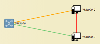
When you put together the JSON files produced by python script in Part II and the D3 visuzalization from Part III, your result on a super-small topology like my LAB will be something like this (using screenshot right now):
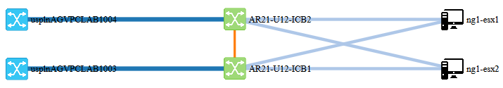
Visualization of LAB topology
Boring, right? Click here for live JavaScript animated demo.
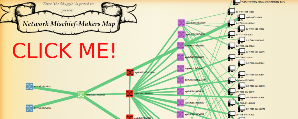
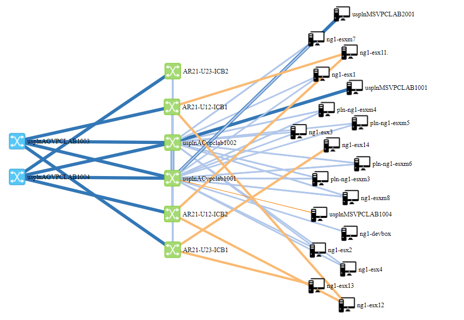
Right, but this is not limited to only my small lab, I actually tried running this in lab at work with a little bit larger device count, this is the result, and again click here for BIGGER live demo.
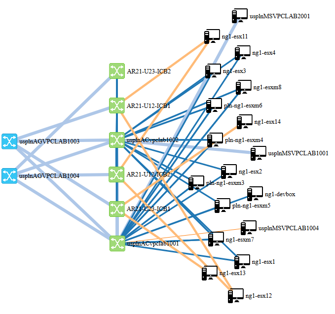
Example of using the shown python/JavaScript visualization on larger LAB
Click here for BIGGER live JavaScript animated demo.
Summary
Well, I shared here with you my quick experiment/example of how to do a quick visualization of network topology using first quick mapping with NETCONF+python+PyHPEcw7 and then visualizing it using Javascript+D3 library to create an interactive, self-organizing map of the topology and some small information pop-ups for each device after clicking on it. You can download the whole project as a package here.